Code Focused Guide on Score-Based Image Models

11 January 2023 · 11 mins

I like inference. Score-based models are possible ways to amortize inference for high-dimensional PPLs.

This is a code focused supplement of Yang Song's blog [ ] on score-based models.

Sampling Densities with Gradients

I'll be writing this in my love language, JAX. Let's do a toy example of learning $p(x)$ first in 2D. Say I gave you this function, which is the log PDF of a donut,

def logpdf(x):
    r = jnp.linalg.norm(x, axis=-1)
    return -(r - 2.6)**2 / 0.033

Figure 0:

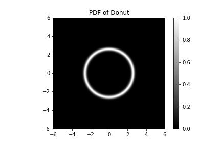
The PDF of our donut plotted. If you look a little closer, we see that the donut hole has a hole in its center - it is not a donut hole at all but a smaller donut with its own hole, and our donut is not a hole at all.

Say we want to draw samples from this PDF. Since this is 2D, it might actually make sense to use rejection sampling, or importance sampling. But they won't scale to high dimensional sampling. We can try MCMC. If we assume we know the gradient of the log distribution, $\nabla_x \log p(x)$ , we can use a Langevin sampler.

Let's first use JAX's autograd to get a function that tells us $\nabla_x \log p(x)$ ,

grad_logpdf = jax.grad(logpdf)

# `grad_logpdf` takes in a single 2D point. We want to be able to
# pass in multiple 2D points for higher throughput.
multi_grad_logpdf = jax.vmap(grad_logpdf, in_axes=(0,))

And then run Langevin dynamics,

x_{t+1} = x_{t} + \epsilon \nabla_x \log p(x) + \sqrt{2 \epsilon} \mathcal{N}(0, I)

@partial(jax.jit, static_argnums=(0,))
def langevin_update(grad_func, current_particles, key, epsilon=1e-2):
    key, subkey = jax.random.split(key)
    noise = jax.random.normal(subkey, current_particles.shape)
    next_particles = (
        current_particles
        + epsilon * grad_func(current_particles)
        + jnp.sqrt(2 * epsilon) * noise
    )
    return next_particles, key


def sample_langevin(grad_func, key, num_steps=1000, num_particles=1000, epsilon=1e-2):
    key, subkey = jax.random.split(key)
    particles = jax.random.normal(subkey, (num_particles, 2))

    for t in range(num_steps):
        particles, key = langevin_update(
            grad_func, particles, key, epsilon=epsilon)

    return particles

key = jax.random.PRNGKey(0)
data = sample_langevin(multi_grad_logpdf, key, num_steps=1000, num_particles=10000)

Figure 0:

Langevin Samples from our Donut

Approximating Score Function

Let's say we weren't neatly handed $\nabla_x \log p(x)$ , but instead were just given samples, $\mathcal{D} = \{x_0, x_1, \ldots, x_n\} \sim p(x)$ . From this data we want to learn a neural network $s_\theta(x) \approx \nabla_x \log p(x)$ .

We of course don't have ground truth access to $\nabla_x \log p(x)$ from just $\mathcal{D}$ . Instead we use a technique called score matching. One way to do this is called denoising score matching. Here we pick some noising distribution, $q(\tilde{x} | x)$ , that takes some $x$ and noises it up to $\tilde{x}$ . We then optimize $\theta$ by,

\mathcal{L} = \mathbb{E}_{x \sim p(x), \tilde{x} \sim q(\tilde{x} | x)}\left[\lVert s_\theta(x) - \nabla_{\tilde{x}} \log q(\tilde{x} | x)\right \rVert _2^2]

If we assume $q(\tilde{x} | x) = \mathcal{N}(x, \sigma)$ , then we can analytically get the expression of the gradient, and have a final loss of,

\mathcal{L} = \mathbb{E}_{x \sim p(x), \tilde{x} \sim q(\tilde{x} | x)}\left[\left\lVert s_\theta(x) - \frac{-(\tilde{x} - x)}{\sigma^2} \right\rVert _2^2 \right]

In our code, we will assume data has samples from our donut. We will approximate the score function using small MLP. Note that this MLP takes in a 2D point and returns a 2D gradient.

def score_net_fn(x):
    # Input is a 2D point.
    # Output is a 2D estimate of the gradient.
    mlp = hk.Sequential(
        [
            hk.Linear(32),
            jax.nn.relu,
            hk.Linear(32),
            jax.nn.relu,
            hk.Linear(32),
            jax.nn.relu,
            hk.Linear(2),
        ]
    )

    return mlp(x)

We implement the above loss as,

def denoising_score_match_loss(params, x_original, x_noised, x_noise_sigma):
    scores = score_net.apply(params, x_noised)
    target = -(x_noised - x_original) / x_noise_sigma**2
    return jnp.mean((scores - target) ** 2)

The rest of the training loop,

X_NOISE_SIGMA = 0.1
BATCH_SIZE = 100
NUM_STEPS = 10000


class TrainingState(NamedTuple):
    params: hk.Params
    opt_state: optax.OptState


def sample_batch(batch_size, key):
    key, subkey = jax.random.split(key)

    # Sample a subset of data.
    idx = jax.random.randint(subkey, (batch_size,), 0, data.shape[0])
    x_original = data[idx]

    # Add noise to the data.
    key, subkey = jax.random.split(key)
    x_noised = x_original + jax.random.normal(subkey, x_original.shape) * X_NOISE_SIGMA

    return x_original, x_noised, key

score_net = hk.without_apply_rng(hk.transform(score_net_fn))
params = score_net.init(key, jnp.zeros((BATCH_SIZE, 2)))
optimizer = optax.adam(1e-3)

state = TrainingState(params, optimizer.init(params))

@jax.jit
def update(state, x_original, x_noised):
    grads = jax.grad(denoising_score_match_loss)(
        state.params, x_original, x_noised, X_NOISE_SIGMA
    )
    updates, new_opt_state = optimizer.update(grads, state.opt_state)
    new_params = optax.apply_updates(state.params, updates)
    return TrainingState(new_params, new_opt_state)


for step in range(NUM_STEPS):
    x_original, x_noised, key = sample_batch(BATCH_SIZE, key)
    state = update(state, x_original, x_noised)

    if step % 100 == 0:
        loss = denoising_score_match_loss(
            state.params, x_original, x_noised, X_NOISE_SIGMA
        )
        print(f"Step {step}: loss = {loss}")

Phew, okay, let's run our Langevin sampler on this approximated score function,

def score_grad(x):
    return score_net.apply(state.params, x)

samples = sample_langevin(score_grad, key, num_steps=1000, num_particles=10000)

aaaaanddddd.....

Figure 0:

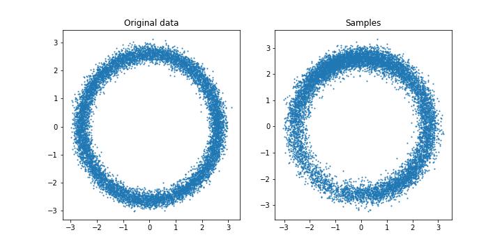
Langevin Samples from our approximated score function.

Yay. Our neural network can learn what the underlying $p(x)$ is from just data. This is pretty sick.

Figure 0:

Visualization of the gradients learned by our neural network.

MNIST and Noise Conditional Score Networks

Learning 2D data is all well and good, but it would be great if we could learn data distributions in high dimensions. Images are great candidates, and of course there is much hype about diffusion and score-based models in the image generation space. I will be using the MNIST dataset. We need two tricks to make this work (1) we need to noise up the images at multiple scales and use annealed Langevin dynamics and (2) our score based approximator should be a U-Net.

I will refer the readers back to Yang Song's blog for the motivation behind why we need multiple scales. Here, I'm just gonna code. When we have multiple noise scales, we have a noise conditional score network, $s_\theta(x, \sigma)$ , which also takes in a $\sigma$ value. This is because $s_\theta(x, \sigma) \approx p_\sigma(x)$ . I will be copying the hyperparameters from the original NCSN work [ ].

Let's first set up our $s_\theta(x, \sigma)$ to be a U-Net. We add the $\sigma$ values as a new channel to the MNIST image. Here is a sloppy and tiny U-Net with skip connections,

NUM_START_FILTERS = 16

def score_net_fn(x_inp, sigmas):
    # Reshape x_inp to 28 x 28.
    x = jnp.reshape(x_inp, (-1, 28, 28, 1))

    # Sigmas are [batch, 1].
    # We need to add sigmas as a channel to x.
    sigmas = jnp.reshape(sigmas, (-1, 1, 1, 1))
    sigmas = jnp.ones_like(x) * sigmas

    # Add sigmas to x as a new channel.
    x = jnp.concatenate([x, sigmas], axis=-1)

    conv1 = hk.Conv2D(NUM_START_FILTERS * 1, (3, 3), padding="SAME")(x)
    conv1 = jax.nn.elu(conv1)
    conv1 = hk.Conv2D(NUM_START_FILTERS * 1, (3, 3), padding="SAME")(conv1)
    conv1 = jax.nn.elu(conv1)
    pool1 = hk.AvgPool((2, 2, 1), (2, 2, 1), padding="VALID")(conv1)

    conv2 = hk.Conv2D(NUM_START_FILTERS * 2, (3, 3), padding="SAME")(pool1)
    conv2 = jax.nn.elu(conv2)
    conv2 = hk.Conv2D(NUM_START_FILTERS * 2, (3, 3), padding="SAME")(conv2)
    conv2 = jax.nn.elu(conv2)
    pool2 = hk.AvgPool((2, 2, 1), (2, 2, 1), padding="VALID")(conv2)

    convm = hk.Conv2D(NUM_START_FILTERS * 4, (3, 3), padding="SAME")(pool2)
    convm = jax.nn.elu(convm)
    convm = hk.Conv2D(NUM_START_FILTERS * 4, (3, 3), padding="SAME")(convm)
    convm = jax.nn.elu(convm)

    deconv2 = hk.Conv2DTranspose(
        NUM_START_FILTERS * 2, (3, 3), stride=(2, 2), padding="SAME"
    )(convm)
    uconv2 = jnp.concatenate([deconv2, conv2], axis=-1)
    uconv2 = hk.Conv2D(NUM_START_FILTERS * 2, (3, 3), padding="SAME")(uconv2)
    uconv2 = jax.nn.elu(uconv2)
    uconv2 = hk.Conv2D(NUM_START_FILTERS * 2, (3, 3), padding="SAME")(uconv2)
    uconv2 = jax.nn.elu(uconv2)

    deconv1 = hk.Conv2DTranspose(
        NUM_START_FILTERS * 1, (3, 3), stride=(2, 2), padding="SAME"
    )(uconv2)
    uconv1 = jnp.concatenate([deconv1, conv1], axis=-1)
    uconv1 = hk.Conv2D(NUM_START_FILTERS * 1, (3, 3), padding="SAME")(uconv1)
    uconv1 = jax.nn.elu(uconv1)
    uconv1 = hk.Conv2D(NUM_START_FILTERS * 1, (3, 3), padding="SAME")(uconv1)
    uconv1 = jax.nn.elu(uconv1)

    output_layer = hk.Conv2D(1, (1, 1), padding="SAME")(uconv1)
    return jnp.reshape(output_layer, (-1, 784))

Then we set up the loss and the noise scales,

NUM_NOISE_SCALES = 10
NOISE_SCALES = [0.63096**scale_index for scale_index in range(NUM_NOISE_SCALES)]


def lambda_(sigma):
    return sigma**2


def denoising_score_match_loss(params, x_original, x_noised, sigmas):
    scores = score_net.apply(params, x_noised, sigmas)
    target = -(x_noised - x_original) / sigmas**2
    squared_error = lambda_(sigmas) * (scores - target) ** 2
    return jnp.mean(squared_error)

And then the rest of the training loop with multiple noise scales.

BATCH_SIZE = 12
NUM_STEPS = 100000


class TrainingState(NamedTuple):
    params: hk.Params
    opt_state: optax.OptState


def sample_batch(batch_size, key):
    rv = []

    key, subkey = jax.random.split(key)
    idx = jax.random.randint(subkey, (batch_size * NUM_NOISE_SCALES,), 0, data.shape[0])
    key, subkey = jax.random.split(key)
    x_original = jnp.reshape(
        data[tuple(idx), :, :], (batch_size * NUM_NOISE_SCALES, -1)
    )
    key, subkey = jax.random.split(key)
    x_noised = (
        x_original
        + jax.random.normal(subkey, x_original.shape)
        * jnp.array(NOISE_SCALES * batch_size)[:, None]
    )
    sigmas = jnp.array(NOISE_SCALES * batch_size)[:, None]

    return x_original, x_noised, sigmas, key


score_net = hk.without_apply_rng(hk.transform(score_net_fn))
params = score_net.init(key, jnp.zeros((BATCH_SIZE, 784)), jnp.ones((BATCH_SIZE, 1)))
optimizer = optax.adam(1e-3)
state = TrainingState(params, optimizer.init(params))

@jax.jit
def update(state, x_original, x_noised, sigmas):
    grads = jax.grad(denoising_score_match_loss)(
        state.params, x_original, x_noised, sigmas
    )
    updates, new_opt_state = optimizer.update(grads, state.opt_state)
    new_params = optax.apply_updates(state.params, updates)
    return TrainingState(new_params, new_opt_state)


for step in range(NUM_STEPS):
    x_original, x_noised, sigmas, key = sample_batch(BATCH_SIZE, key)
    state = update(state, x_original, x_noised, sigmas)

    if step % 100 == 0:
        loss = denoising_score_match_loss(state.params, x_original, x_noised, sigmas)
        print(f"Step {step}: loss = {loss}")

Here is an example of a batch we pulled, and how different noise scales have corrupted the image,

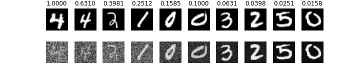
Batch for Multi-Scale Denoising Score Matching

Figure 0:

Example of a batch pulled. Here we see how different noise scales (sigma values on the top) perturb the original image (top row) into the noisy versions (bottom row).

To sample, we need to use an annealed Langevin sampler, where we slowly start the conditional score function, $s_\theta(x, \sigma)$ at a high $\sigma$ and reduce it to the lowest noise scale.

def score_grad(x, sigma):
    batch_size = x.shape[0]
    sigmas = sigma * jnp.ones((batch_size, 1))
    return score_net.apply(state.params, x, sigmas)


@jax.jit
def langevin_update_annealed(current_particles, key, sigma, alpha):
    key, subkey = jax.random.split(key)
    z_t = jax.random.normal(subkey, current_particles.shape)
    particles = (
        current_particles
        + alpha / 2 * score_grad(current_particles, sigma)
        + jnp.sqrt(alpha) * z_t
    )
    return particles, key


def sample_langevin_annealed(
    key, num_steps=1000, num_particles=1000, eta=1e-2, dim=2, init_particles=None
):
    key, subkey = jax.random.split(key)

    if init_particles is None:
        particles = jax.random.normal(subkey, (num_particles, dim))
    else:
        particles = init_particles

    sigma_L = NOISE_SCALES[-1]
    for i in range(NUM_NOISE_SCALES):
        sigma_i = NOISE_SCALES[i]
        alpha_i = eta * sigma_i**2 / sigma_L**2

        for t in range(num_steps):
            particles, key = langevin_update_annealed(particles, key, sigma_i, alpha_i)

    return particles

samples = sample_langevin_annealed(
    key, dim=784, num_steps=100, eta=2e-5,
    init_particles=jax.random.uniform(jax.random.PRNGKey(0), (10, 784), minval=0, maxval=1)
)

aaaaanddddd.....??

Figure 0: Samples from our score-based MNIST model.

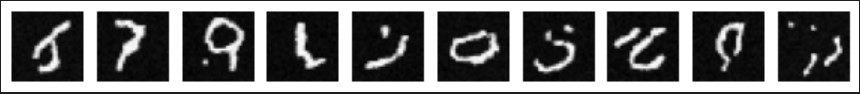
Kinda look like digits lol? I think making the U-Net much bigger and having best practices could improve the quality substantially.

References

Shreyas Kapur's Blog

srkp@berkeley.edu

Home Projects Blogs