Neural Density Estimation via Diffusion

1 July 2024 · 9 mins

Say you have a bunch of data, $\mathcal{D} = \{x_1, x_2, \ldots, x_n\}$ . Where $x_i \in \mathbb{R}^d$ , and $x_i \sim p(x)$ . In the GenAI™ paradigm, we typically want to sample more data from $p(x)$ . Typically, $x$ 's could look like images, or audio, etc. At the time of writing diffusion models [ ] would be the best. But very often we don't care about sampling, we care about density estimation. We want to know the value of $p(x)$ at a particular $x$ . Questions like, "what is the density of the image?" are common in practice for tasks like anomaly detection, or uncertainty estimation.

In this post, I'll show you how to estimate the density of $p(x)$ , using diffusion models, but not using diffusion models. We will train a bunch of classifiers that learn to estimate the density by adding noise to your dataset, and then combine them to estimate the density. This is a very simple method to implement and seems to work quite well.

Problem Setup

Let's work with our trusty donut density,

def logpdf(x):
    r = np.linalg.norm(x, axis=-1)
    return -(r - 2.6)**2 / 0.033

Which looks like this,

Figure 0:

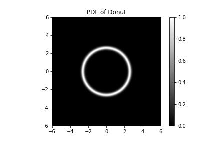
The PDF of our donut plotted. If you look a little closer, we see that the donut hole has a hole in its center - it is not a donut hole at all but a smaller donut with its own hole, and our donut is not a hole at all.

Let's generate some data from this distribution,

Figure 0:

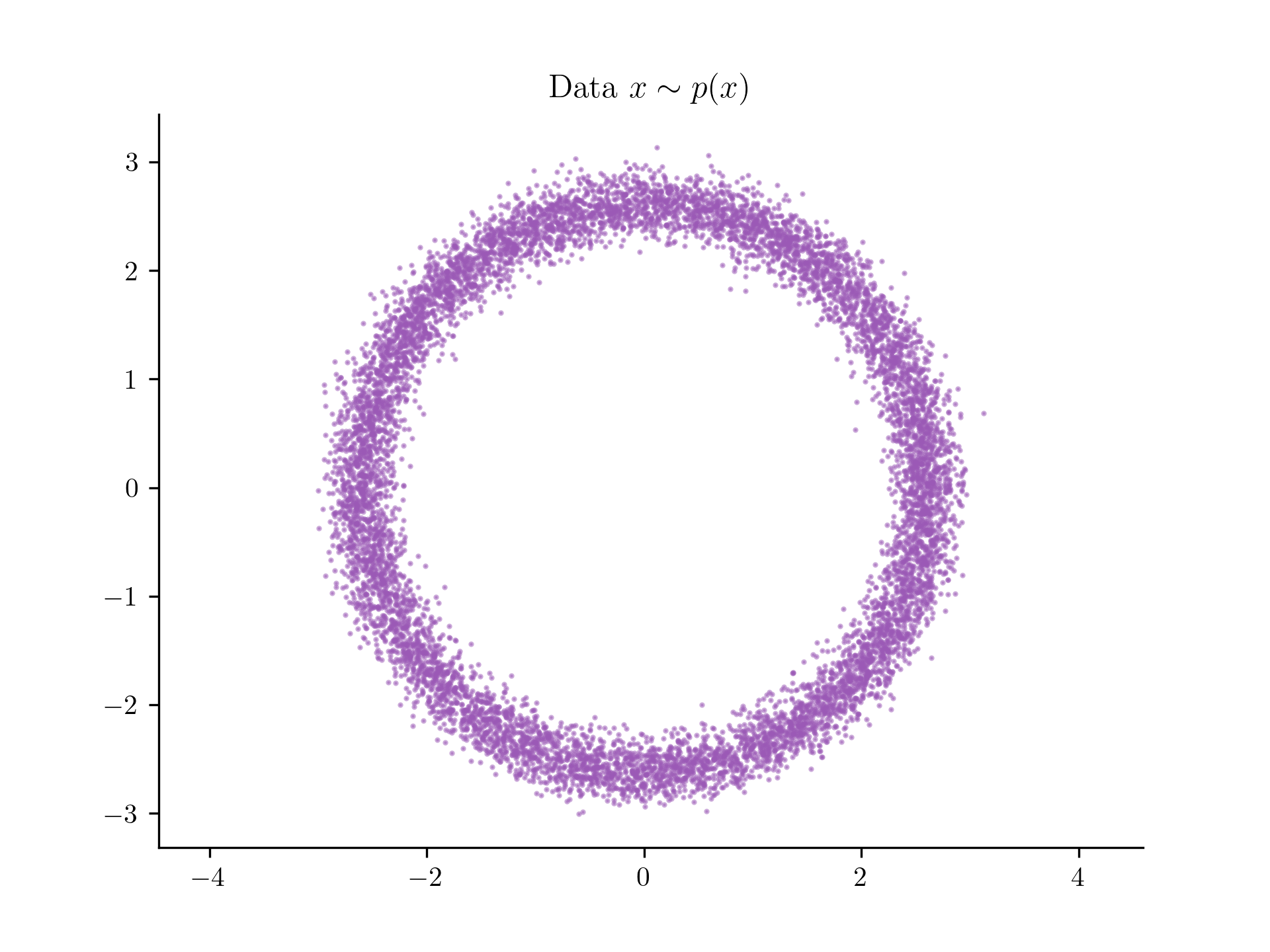
The dataset we'll be working with.

As you can see we have $x \in \mathbb{R}^2$ , and we have a dataset of $n=10000$ examples. Our goal is to be able to evaluate the density of $p(x)$ at any point $x$ , using only this dataset, $\mathcal{D} = \{x_1, x_2, \ldots, x_n\}$ .

Density Estimation via Classification

In the most basic setup, we can train a neural network to learn this density from this dataset by simply doing classification. We will train a neural network to classify whether a point is coming from $\mathcal{D}$ or another dataset $\mathcal{D}'$ . This $\mathcal{D}'$ is generated from a distribution that is very easy to sample from, like a Gaussian or a uniform distribution. We can train this neural network to simply do binary classification, and then use the output of this network to estimate the density.

Our dataset $\mathcal{D} \sim p(x)$
Our proposal distribution $\mathcal{D}' \sim q(x)$

Let $d_\theta(x)$ be a neural network that models the probability that point $x$ came from either $p(x)$ or $q(x)$ . We can write this as,

\begin{align} d_\theta(x) &= p(x \sim p(x) \ \text{or} \ x \sim q(x)) \\ &= \frac{p(x)}{p(x) + q(x)} \end{align}

\implies p(x) = \frac{d_\theta(x)}{1 - d_\theta(x)} q(x). \tag{1}

Using Equation 1, we can estimate the density of $p(x)$ at any point $x$ by evaluating $d_\theta(x)$ at that point. We can train $d_\theta(x)$ by minimizing the binary cross-entropy loss. Let's pick $q(x)$ to be a Uniform distribution over the range $[-5, 5] \times [-5, 5]$ . We can generate a dataset $\mathcal{D}'$ from this distribution.

Figure 0:

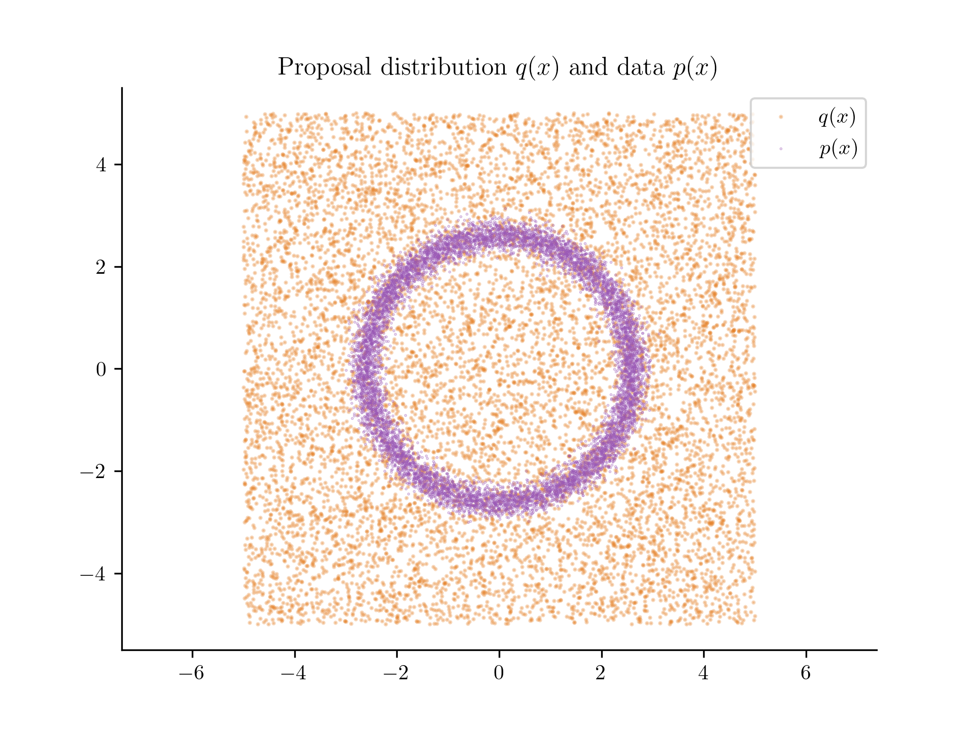
The proposal distribution (in orange) and the data points (in blue).

For numerical stability, we will actually train things using the following logistic loss from [ ],

\mathcal{L}_\theta = -\mathbb{E}_{x \sim p(x)} \log\left(\frac{d_\theta(x)}{1 + d_\theta(x)}\right) -\mathbb{E}_{x \sim q(x)} \log\left(\frac{1}{1 + d_\theta(x)}\right). \tag{2}

This loss will estimate the density ratio between $p(x)$ and $q(x)$ ,

d_\theta(x) = \frac{p(x)}{q(x)}.

Where $d_\theta(x)$ is the output of the neural network with an additional exponential transformation. This is done to ensure that the output of the neural network is always positive.

Now, our task for the neural network is to classify whether a point is coming from the blue distribution or the orange distribution.

Let's define our neural network,

class DensityModel(nn.Module):
    def __init__(self):
        super(DensityModel, self).__init__()
        self.fc1 = nn.Linear(2, 128)
        self.fc2 = nn.Linear(128, 128)
        self.fc3 = nn.Linear(128, 1)

    def forward(self, x):
        x = F.relu(self.fc1(x))
        x = F.relu(self.fc2(x))
        return self.fc3(x)

This takes in a point $x \in \mathbb{R}^2$ and outputs a single value.

We can then train using the following code,

batch_size = 128
num_steps = 10000

def sample_batch():
    data_idx = np.random.choice(len(data), batch_size // 2)
    proposal_idx = np.random.choice(len(proposal_dataset), batch_size // 2)

    data_batch = torch.tensor(data[data_idx], dtype=torch.float32)
    proposal_batch = torch.tensor(proposal_dataset[proposal_idx], dtype=torch.float32)

    return torch.cat([data_batch, proposal_batch], dim=0)

def loss_fn(model, x):
    ratios = torch.exp(model(x))
    ratios_p = ratios[:batch_size // 2]
    ratios_q = ratios[batch_size // 2:]
    return torch.mean(-torch.log(ratios_p / (ratios_p + 1)) - torch.log(1 / (ratios_q + 1)))

model = DensityModel()
optimizer = optim.Adam(model.parameters(), lr=1e-3)

for step in range(num_steps):
    optimizer.zero_grad()
    x = sample_batch()
    loss = loss_fn(model, x)
    loss.backward()
    optimizer.step()

    if step % 100 == 0:
        print(f"Step {step}, loss: {loss.item()}")

Once the model is learned, we can get the predicted value of $\frac{p(x)}{q(x)}$ by evaluating the model at $x$ and exponentiating the output,

\frac{p(x)}{q(x)} = \exp(d_\theta(x)).

In this case $q(x)$ is a uniform, which is a constant. So $p(x) \propto \exp(d_\theta(x))$ . We can then plot the density of $p(x)$ at any point $x$ , by just calling the model at that point.

Figure 0:

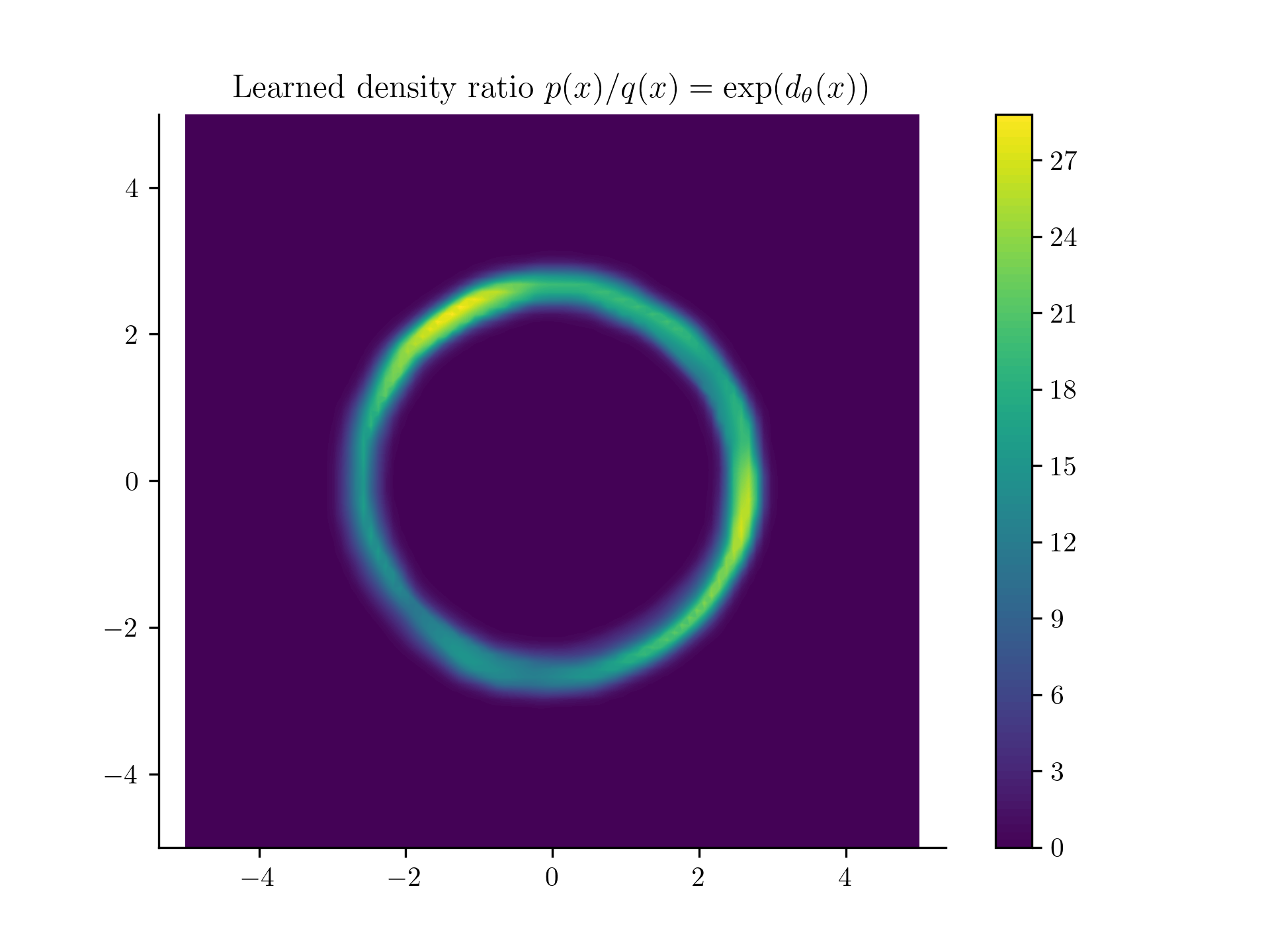
Our learned density from samples!

This doesn't look too bad! Next we'll see the problems with this approach and how to fix them.

Problems with Density Estimation via Classification

Recall that $p(x)$ is the density we want to learn and we picked an easy density $q(x)$ to help us train our classifier. We picked $q(x)$ to be a uniform distribution over the range $[-5, 5] \times [-5, 5]$ . What if we picked a different $q(x)$ ? Would our classifier still work?

Figure 0:

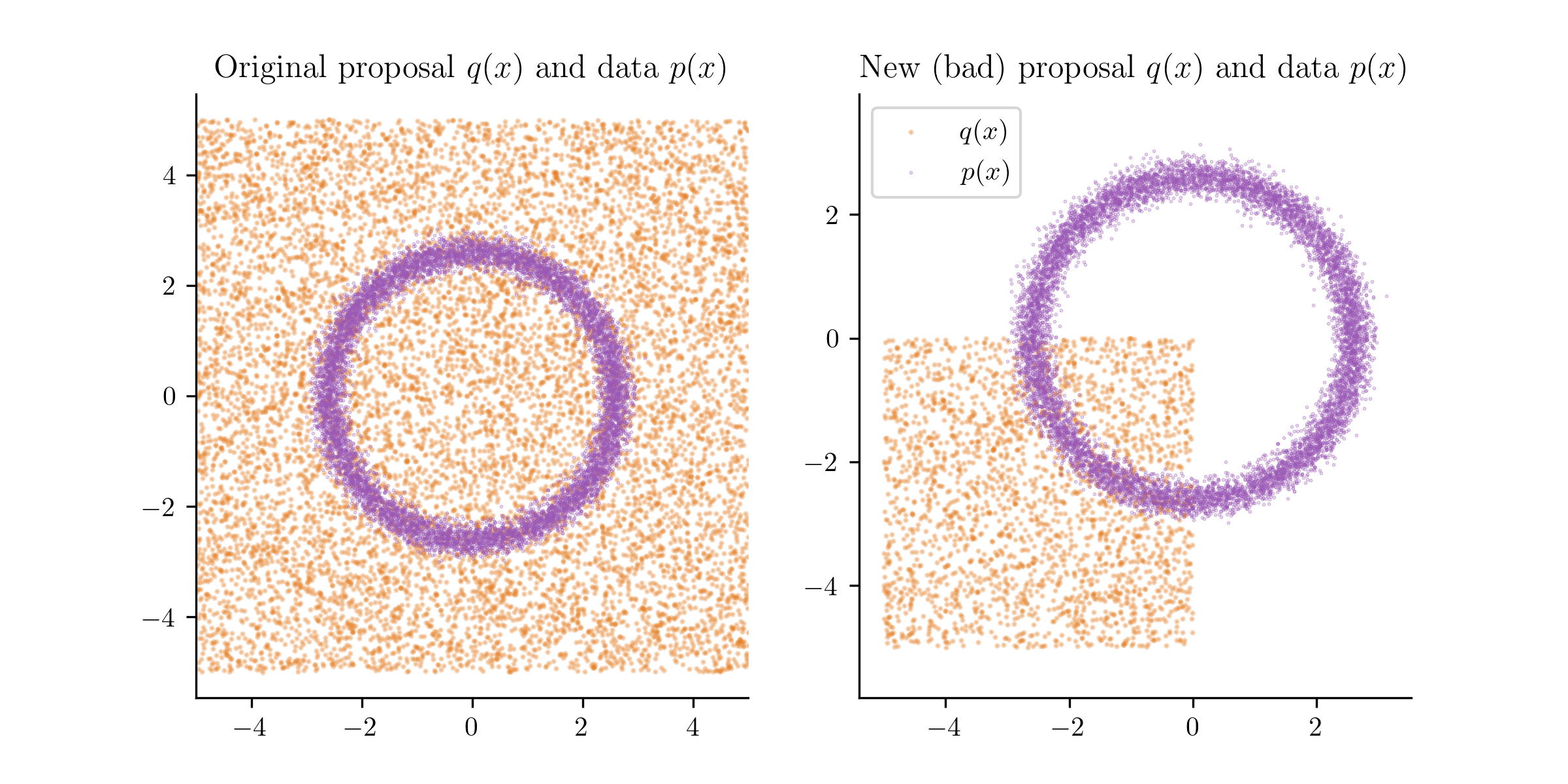
The new proposal distribution (in orange) and the data points (in blue).

Above, I show a new $q(x)$ which is a uniform over the range $[-5, 0] \times [-5, 0]$ . If we train our classifier on this new $q(x)$ , we will get a very different density estimate,

Figure 0:

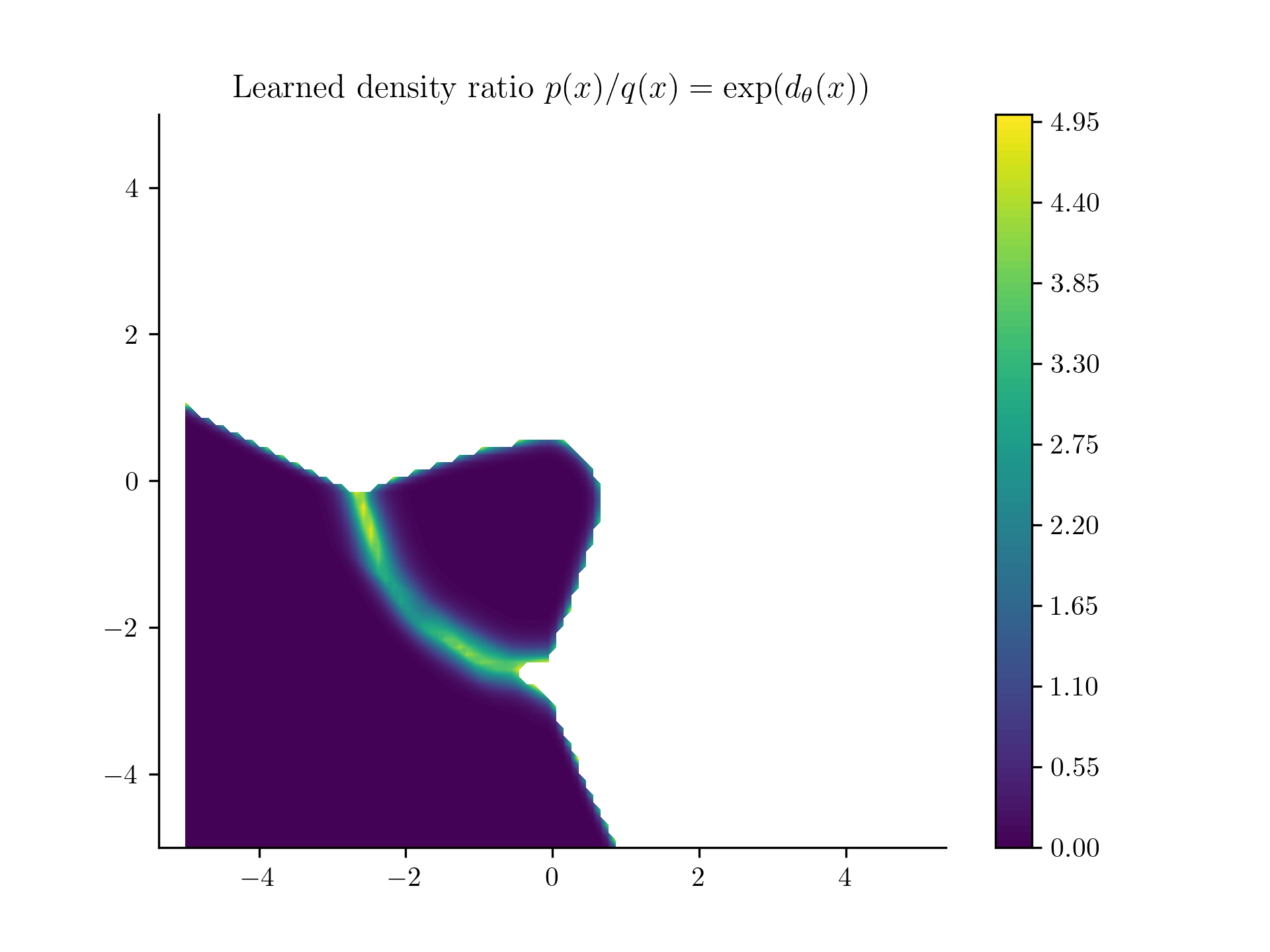
Yeah, that's sad. White values were basically NaNs.

What's happening here? In the lower-left quadrant, classifiying between the orange $q(x)$ points and the blue $p(x)$ points is an interesting problem. But on all the other quadrants, the task is too easy. The classifier can just learn to classify all points in that upper region as $p(x)$ , even though that is not true. We simply don't have enough contrasting data for those points. So the choice of $q(x)$ is very important.

Diffusion To The Rescue!

I'm mashing together the ideas from [ ] and [ ] here. We can fix the problem of choosing $q(x)$ by ... just adding noise to our dataset! We can train a classifier to classify whether a point is coming from the original dataset $\mathcal{D}$ or a noisy version of the dataset $\mathcal{D}_\epsilon$ . We can then use the output of this classifier to estimate the density of $p(x)$ . But this is still bad, because if we add too much noise to our dataset, we again have a very easy classification problem (think about making a density estimator for images, it is very easy to classify between gaussian noise and an image).

Instead, we'll incrementally add noise, just like in diffusion or score-based models.

Let $p_0(x)$ be our original density. We will generate a sequence of densities $p_1(x), p_2(x), \ldots, p_T(x)$ by adding higher and higher amounts of noise to our dataset. For simplicity, we will add Gaussian noise to our dataset,

p_i(x) = p_0(x) + \sigma_i \mathcal{N}(0, 1).

Here $\sigma_i$ is some noise schedule that tells us the amount of noise for level $i$ . We can then train a classifier to classify whether a point is coming from $p_i(x)$ or $p_{i+1}(x)$ . So,

\frac{p_i(x)}{p_{i+1}(x)} = \exp(d_\theta(x, \sigma_i)).

Note that our model now gets an additional input, the noise level $\sigma_i$ , which tells the model which classification problem it's working on. To estimate the density of $p_0(x)$ , we can use the telescoping product,

\begin{align*} \frac{p_0(x)}{p_T(x)} &= \frac{p_0(x)}{\cancel{p_1(x)}} \frac{\cancel{p_1(x)}}{\cancel{p_2(x)}} \ldots \frac{\cancel{p_{T-1}(x)}}{p_T(x)} \\ &= \exp(d_\theta(x, \sigma_0) + d_\theta(x, \sigma_1) + \ldots + d_\theta(x, \sigma_{T-1})). \end{align*}

This method is has analogies to Simulated Annealing and the Langevin Monte Carlo method.

Okay! Let's implement this in code.

NUM_NOISE_SCALES = 10
NOISE_SCALES = [0.63096**scale_index for scale_index in range(NUM_NOISE_SCALES)][::-1]
FULL_NOISE_SCALES = np.array([0] + NOISE_SCALES)

for i, noise_scale in enumerate(FULL_NOISE_SCALES):
    noised_data = data + np.random.normal(0, noise_scale, data.shape)
    # Plot the noised data.
    # ...

Figure 0:

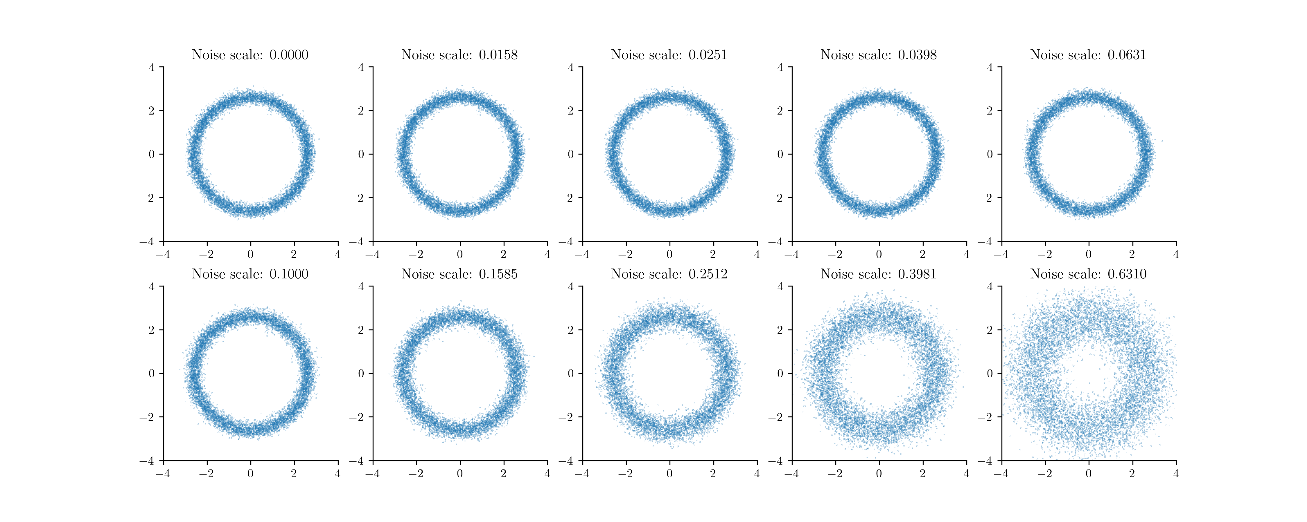
Our incremental distributions for the donut.

Let's modify out model so it takes in a $x \in \mathbb{R}^2$ and a noise level $\sigma_i$ ,

class DensityModel(nn.Module):
    def __init__(self):
        super(DensityModel, self).__init__()
        self.fc1 = nn.Linear(3, 128)
        self.fc2 = nn.Linear(128, 128)
        self.fc3 = nn.Linear(128, 1)

    def forward(self, x, sigmas):
        # x.shape = (batch_size, 2)
        # sigmas.shape = (batch_size, 1)
        # Concatenate the sigmas to the input to get a (batch_size, 3) tensor.
        x = torch.cat([x, sigmas], dim=1)
        x = F.relu(self.fc1(x))
        x = F.relu(self.fc2(x))
        return self.fc3(x)

We can then train the model using the following code,

batch_size = 128
num_steps = 10000

def sample_batch():
    noise_levels = np.random.randint(0, NUM_NOISE_SCALES, batch_size // 2)

    pre_sigmas = FULL_NOISE_SCALES[noise_levels]
    post_sigmas = FULL_NOISE_SCALES[noise_levels + 1]
    
    data_idx_pre = np.random.choice(len(data), batch_size // 2)
    data_batch_pre = data[data_idx_pre]

    data_idx_post = np.random.choice(len(data), batch_size // 2)
    data_batch_post = data[data_idx_post]

    pre_data = data_batch_pre + np.random.normal(0, pre_sigmas[:, None], data_batch_pre.shape)
    post_data = data_batch_post + np.random.normal(0, post_sigmas[:, None], data_batch_post.shape)

    data_batch = np.concatenate([pre_data, post_data], axis=0)
    sigmas = np.concatenate([post_sigmas, post_sigmas], axis=0)
    return torch.tensor(data_batch, dtype=torch.float32), torch.tensor(sigmas, dtype=torch.float32)[:, None]


def loss_fn(model, x, sigmas):
    ratios = torch.exp(model(x, sigmas))
    ratios_p = ratios[:batch_size // 2]
    ratios_q = ratios[batch_size // 2:]
    return torch.mean(-torch.log(ratios_p / (ratios_p + 1)) - torch.log(1 / (ratios_q + 1)))

model = DensityModel()
optimizer = optim.Adam(model.parameters(), lr=1e-3)

for step in range(num_steps):
    optimizer.zero_grad()
    x, sigmas = sample_batch()
    loss = loss_fn(model, x, sigmas)
    loss.backward()
    optimizer.step()

    if step % 100 == 0:
        print(f"Step {step}, loss: {loss.item()}")

And .. drumroll please,

Figure 0:

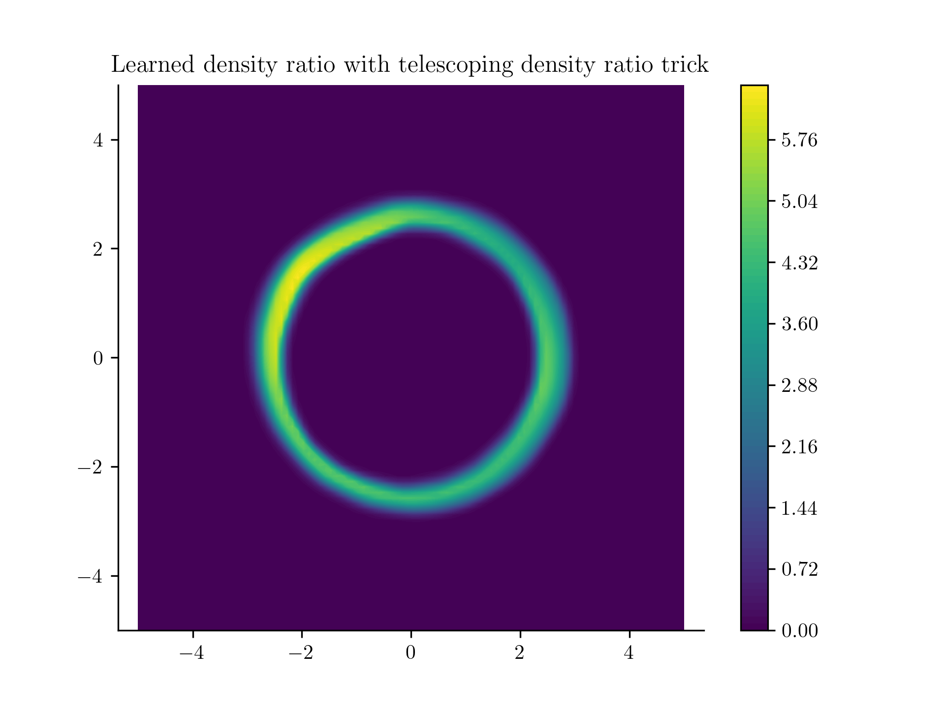
Learned density using the incremental noise levels!

Here is a little animation of it learning,

Figure 0:

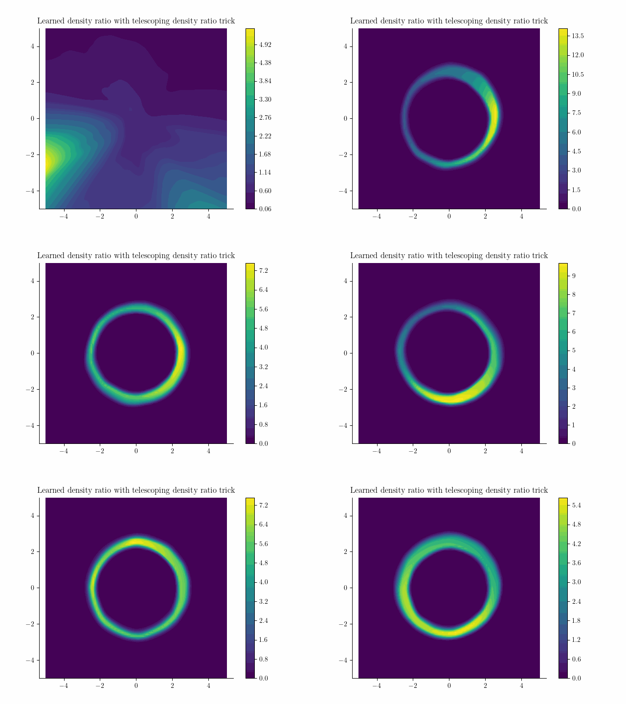
Learned density using the incremental noise levels!

You can find the full code for this blog post here.

Citation

@misc{kapur2024density,
  url={https://shreyaskapur.com/blogs/density},
  journal={Neural Density Estimation via Diffusion},
  author={Kapur, Shreyas},
  year={2024},
  month={Jul}
}

References

Shreyas Kapur's Blog

srkp@berkeley.edu

Home Projects Blogs